Ballpark Pal Methods

Introduction

Ballpark Pal produces in-depth projections for every MLB game, utilizing a system that can be thought of more as a collection of models than a single predictive formula. At its core is the understanding that baseball is a game that unfolds as a series of random events. Though these events are shaped by player abilities, they're strongly influenced by external factors such as stadium variation, weather, batted ball luck, and the general randomness that comes from small samples. Our chosen approach focuses on separating player abilities from outside influences, largely through machine learning and simulations. Below is a comprehensive breakdown of the projection system, explaining each component and its role in creating the daily content you see on the site.

Randomness and External Factors

From a game-to-game basis, it's easy to make the argument that baseball is the most random of the major professional sports. The obvious factor is the playing field, which is different depending on the city. A 102-mph fly ball exiting the bat at 32° in Cincinnati is often a sure homer, while it's normally a routine flyout in Detroit. A soft bloop in the tight confines of Seattle may usually be a flyout but can easily fall for a base hit in the spacious Kansas City outfield.

Even the conditions within a stadium can vary sharply between games. A simple shift of the wind at Wrigley can make the difference between a pitcher's duel and a 15-run game. And the results of a contest played in Cleveland's July weather might be vastly different than if it were 50° in April when the ball doesn't carry as far.

But there are lots of random factors built into baseball that have nothing to do with the environment or skill level of the players. A 115-mph rocket off the bat could be an out or a double depending on the exact position of the third baseman. An 88-mph meatball thrown over the heart of the plate could result in a 480-foot bomb or a routine strike, depending on if the batter decides to swing on 3-0.

Contrast this phenomenon with a sport like basketball in which a particular 3-pointer, regardless of the circumstances, will always fall through the hoop if it leaves the shooter's hand in a certain way. Fortunately, there are 162 games for all the randomness and external effects to fall on each side of the luck spectrum. But even then, you have teams playing half their games in a single park and a large portion of games against their own division and league. Not to mention that games played 6 months or even 6 weeks ago can easily become outdated from a predictive standpoint.

Expectation Models

The most fundamental component of Ballpark Pal projections is that they're largely based on expected outcomes, not the actual results that occur on the field. Our system uses the physical characteristics of every pitch and every batted ball to assign a prediction or expectation of what the outcome should be.

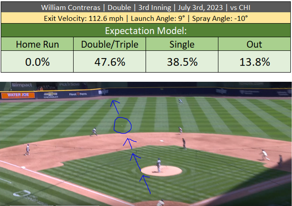
Batted Ball Example #1: William Contreras smokes a line-drive double through the infield at 112 mph. Based on how the ball left the bat, the expectation model gave it a 47.6% chance of being a double or triple, 38.5% chance of being a single, and 13.8% chance of being an out.
Batted Ball Example #2: Randy Arozarena hits a sharp line drive to left-center. The ball comes up several feet short of a homer and falls into Jarred Kelenic's glove, who has to leap at the warning track to catch it. Based on how the ball left the bat, the expectation model gave it a 64.2% chance of a home run, 24.8% chance of a double or triple, and just a 7.9% chance of an out.
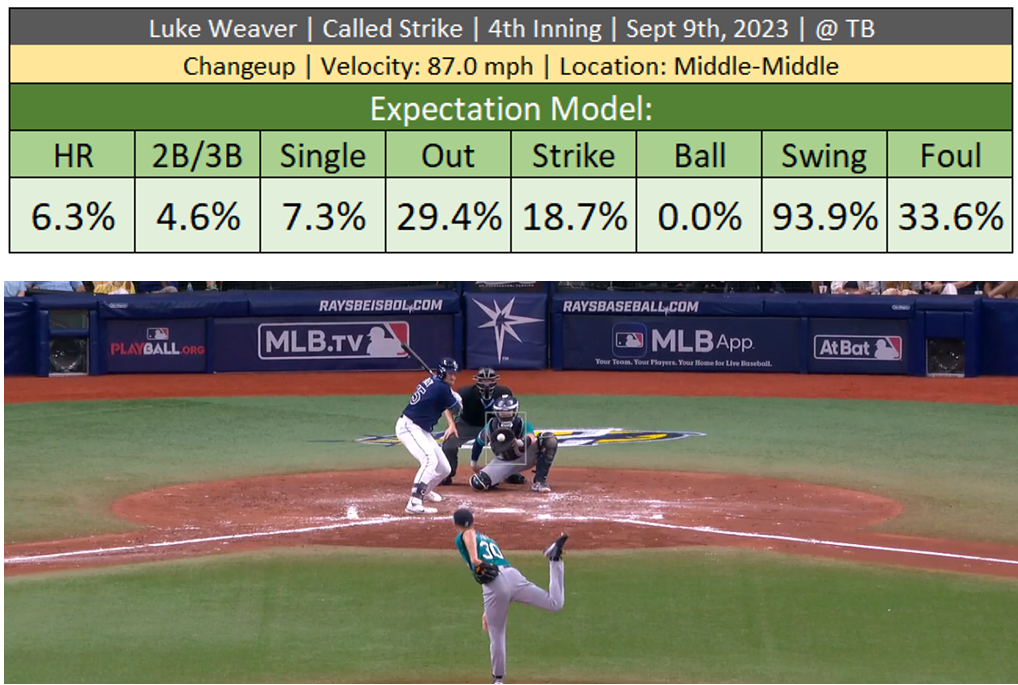
Pitch Example #1: Luke Weaver throws Luke Raley an 87 mph changeup right down the middle on a 2-1 count. Based on the location, situation, and physical characteristics of the pitch, the expectation model assigns an 18.2% chance of a hit and a whopping 6.3% chance of a home run. Raley takes the pitch for strike two despite how poor the pitch was.
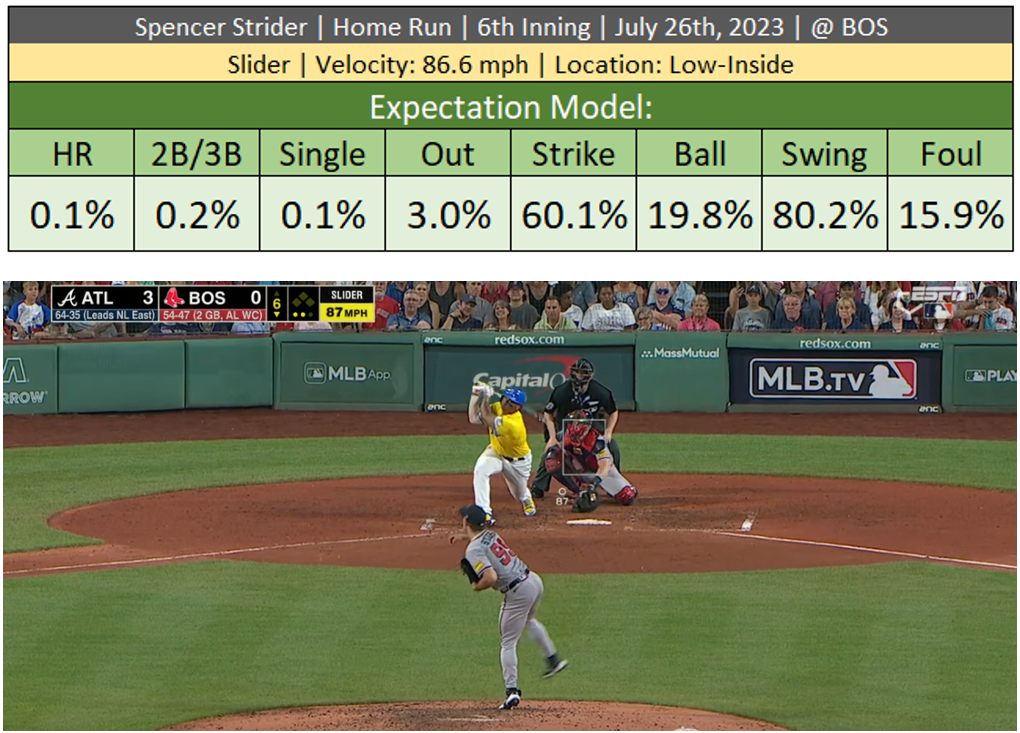
Pitch Example #2: Spencer Strider throws a wicked slider down and inside to Rafael Devers on a 1-2 count. Based on the location, situation, and physical characteristics of the pitch, the expectation model assigns less than 1% chance of a hit and a 60% chance of a swing-and-miss. Devers somehow golfs the slider over the right field wall.

Assigning an expected outcome to a pitch involves examining its physical aspects. How fast was it? How much did it break? How fast did it spin? Where did it cross the plate? Etc. The way that we're able to determine which factors are most important (and how they interact with one another) is by training a model over a large dataset of historical pitches. This method utilizes machine learning, which is a common technique for predicting an outcome from a large set of complicated and interdependent factors. The pitch expectation model is trained over a dataset of 5 million pitches since 2016. Here's a small subset of some of the basic features accounted for in the model: It was apparent early on in developing this model that physical characteristics combined with situational info wasn't enough to fully account for the differences between pitchers. In other words, two pitchers throwing the exact same pitch can often expect different outcomes based on their delivery, pitch sequencing, complementary arsenal, number of pitch types, knowledge of the batter's tendencies, or other soft factors they use to their advantage. Therefore, the model also tries to account for some of these important hidden differences by using features like the ones listed below. For every pitch in the training data, these types of variables are referenced alongside its physical characteristics to provide context about the pitcher's full arsenal and softer skill set. One of the trickiest and most important aspects of MLB projections is determining the skill level of pitchers, which can easily be masked by randomness (especially in the short term). The Pitch Model plays an important role in determining the repeatability of a pitcher's outcomes based on how effective his pitches appear.

Ballpark Pal also assigns expectations to batted balls according to how they exit the bat. Like pitches, the physical aspects of a ball put in play such as exit velocity, launch angle, and direction are more indicative of the hitter's skill level than its actual result on the field. The main idea is that a hitter should be rewarded for a well-hit ball regardless of the circumstances surrounding it. Whether it ends up as a home run during a hot day at Coors Field or a flyout during a cold evening at Oracle Park should be irrelevant in forecasting that player's future performance. Similarly, he shouldn't be rewarded for barely clearing the right field wall at Yankee Stadium if that's the only park that would have failed to contain it.

The model responsible for making these predictions is trained over a dataset of 800,000 balls put in play since 2016. The most important factors are exit velocity, launch angle, and spray angle (direction). However, there are some important nuances the model uses that may not seem obvious. For instance, pulled fly balls travel farther than those hit to the opposite field even if they leave the bat the exact same way. Presumably this has to do with the additional backspin produced by a pulled fly ball that allows it to carry farther. Similarly, the type and location of the pitch also contribute to the distance traveled (and therefore the outcome) in addition to how the ball exits the bat. Here is a list of factors this model uses to assign expected outcomes. This model isn't only important for measuring the raw abilities of players, but also helps establish a baseline for other tasks such as quantifying stadium effects. I'll refer to it as the Contact Model (or "C-Only" model) for the rest of the guide as it's focused solely on how the ball leaves the bat.

Parks and Weather

So far, this guide has focused on the importance of removing external factors from the equation to more accurately gauge player abilities. But when it comes to parks and weather, it's necessary to put the outside elements back in the equation to account for the game's venue and weather forecast.

To help determine how much external stuff to put back in, we train a new variation of the Contact Model, but instead of restricting its knowledge to how the ball left the bat, we also allow insight into the environment. Here are the factors this new model uses to make predictions, with the added variables highlighted in green. Like most of the models discussed in this guide, this one is smart enough to detect local effects and nuanced interactions between the variables, which is especially important for park factors. This feature allows us to detect that wind speed matters the most at Wrigley and hardly at all in places like Milwaukee and Toronto where the tall stadium walls effectively block the wind from entering the venue.

So now we have a "Contact" Model (C-Only) and a "Contact + Park + Weather" model (CPW). These two models working in conjunction are the basis for measuring park factors. Here's an example to demonstrate:

It's a humid, 85° day at Yankee Stadium with the wind blowing out to center at 10-mph. Anthony Rizzo pulls a high fly ball down the right field line. Rizzo gets under it and the glorified pop up manages to barely clear the notorious short porch for a homer.

C-Only Model: Based on the high launch angle and soft contact, and without knowledge of the environment, Rizzo's fly ball has a 25% chance of being a home run in the direction it was hit.

CPW Model: Rizzo's fly ball left the bat at a high launch angle with relatively soft contact. But since hitting conditions are favorable and because right field at Yankee Stadium is particularly shallow, that fly ball has a 75% chance of being a home run.

To assign credit to the environment, we subtract the C-Only probability from the CPW probability:

By comparing the output of two separate models, one with restricted information and one with full knowledge, we're able to make a reasonable guess about how much the difference between the models (park and weather) contributed to the fly ball's outcome.

The park factors that Ballpark Pal publishes on a game-by-game basis originate at the batter level. This is important because the layout of the stadium and the nature of the day's weather will affect each player's batted ball profile differently. For example, Alex Bregman and Yordan Alvarez both play their home games in Houston, but Minute Maid Park tends to favor Bregman more. While Alvarez hits a decent portion of his barrels toward the deep center field fence, Bregman tends to pull his fly balls toward the shallow Crawford boxes in left. Here's a basic example of how park factors may be assigned to players for an individual game played at Minute Maid Park: First we establish a batted profile for each player using their history. We grade each of the batted balls with the C-Only model to determine how many home runs the hitter is expected to have while ignoring the park and environmental effects (C-Only HR). Then we evaluate each batted ball using the CPW model with inputs from today's weather forecast and venue (CPW HR). To get the final park factor for each player, we compare the CPW estimate to the C-Only estimate.

As shown in the chart above, Bregman's tendency to hit his fly balls to left makes the Astros home venue a favorable park for him. Alvarez on the other hand hits a good portion of his fly balls to center, which is more difficult due to the deeper-than-average fence in that direction. His park factor turns out negative in this example case since he'd be expected to hit more home runs in other stadiums.

The approach just described effectively deals with park-to-park and day-to-day variation related to flight of the ball after contacting the bat. However, stadiums don't just impact the game when the ball is put in play. Believe it or not, there are real differences between parks when it comes to the rate and quality of contact allowed. These effects are tricky to detect and involve sifting through noise associated with home/away splits (a technique that won't be detailed in this guide). While it's next to impossible to pinpoint the cause of these differences, here are a few factors we can guess are responsible to some degree.

Batter's eye variation: The open area behind the center field fence serves as a visual backdrop for the baseball as it leaves the pitcher's hand and travels toward home plate. This area looks different depending on the park and some parks may cause more visual interference than others.

Altitude effect on pitch movement: Pitching at Coors Field isn't just difficult because the ball flies farther. The higher altitude also reduces the amount that pitches break, and straighter pitches are easier for batters to hit. This is mostly just a Coors phenomenon but there could be similar impacts elsewhere such as Arizona and Atlanta, which are two of the highest elevated MLB cities outside of Denver.

Mound variation: There is some evidence that the pitching mound varies slightly from park to park, both in height and construction/maintenance. As a result, certain mounds may be slightly more conducive to pitching than others.

Backstop distance: The distance from home plate to the first row of seats varies across parks. It's possible that the different aesthetic has a small effect on how well pitchers execute their pitches.

Effect of outfield size on hitting approach: There is an interesting phenomenon in that rate and quality of contact is better for parks with spacious outfields and worse for parks where the fence is closer to home plate. This may be due to hitters changing their approach to fit the venue. For example, they may be more likely to swing for the short fences in Cincinnati and simply try to put the ball in play in Kansas City where the large outfield is more difficult to cover.

To recap, there are three factors that Ballpark Pal uses to adjust for park factors.

1) Post-contact flight of the ball
2) Contact rate
3) Contact quality

Let's revisit the Bregman/Alvarez example to demonstrate how these aspects are combined to calculate park factors for a given hitter on a given day.

As you navigate the site, you'll see park factors assigned to each game on the slate. Since the simulations use batter-level park factors, these are provided simply for illustrative purposes. To calculate these game-level factors, we apply a weighted average to the players in each lineup according to each hitter's expected number of plate appearances. Next to evaluating pitchers, accurately accounting for park factors is perhaps the trickiest and most important aspect of MLB forecasting. It's easy to conflate a park's tendencies with its home team's abilities, especially in extreme cases when the lineup is loaded and/or the pitching is notably poor. The approach of using expected outcome models separates park effects from the skill levels of players. It naturally accounts for the differences in field dimensions, varying effects of weather, and diverse batted ball profiles across hitters.

Matchup Model

Much has been made in this guide about how random baseball is, but one aspect that makes it more convenient to forecast relative to other sports is the independent nature of player matchups. Two basketball players may guard one another for a decent portion of the game, but they won't be attached at the hip and often won't even be on the court at the same time. In football, a defensive back might be assigned to cover a particular receiver, but his attention will naturally shift to other assignments throughout the game. Sports like soccer and hockey are free-flowing with lots of moving parts and are hardly based on two opposing players matching up directly.

Baseball is the rare instance in which two players, a batter and pitcher, face off directly. It isn't quite as clean as a tennis match since outside forces like baserunners, the catcher, the on-deck hitter, and other things still have an impact. But the fact that outside factors are largely separated makes predicting the outcome a relatively straightforward task, at least compared to what's been discussed to this point.

The purpose of the matchup model is to facilitate game simulations. As discussed in the next section, simulations rely on probabilities to effectively capture an expected range of outcomes. Therefore, predicting the result of a batter/pitcher matchup isn't a matter of choosing a particular outcome such as a single, flyout, or home run. Instead, we assign a probability to each of the possible outcomes. This model's objective is to generate probability distributions for every batter/pitcher combination that are as realistic and accurate as possible. The table above shows the desired output. Each batter/pitcher matchup is assigned a probability distribution that adds up to 100%. To get to this point, we train a machine learning model over a dataset of over 1 million plate appearances since 2016. While technical aspects such as model architecture and training parameters are important, the key factor dictating prediction accuracy is the set of variables used in training.

The current version of the matchup model has over 100 distinct variables, each of which are highly engineered. In other words, they don't exactly resemble a FanGraphs stat line. In fact, every "stat" that goes into the model is proprietary and developed internally. The model has no knowledge of traditional advanced metrics such as wRC+, xwOBA, OBP, BABIP, WAR, FIP, OPS+, ISO, Barrel %, or other stats that are well known to the analytics community. This is because developing predictive signals for machine learning is a different task than creating digestible stats for humans. Most of the features are derived from expectation models (as discussed toward the beginning of this guide) and aren't easy to explain in a few sentences or capture in a single formula. Although not an exhaustive list of each variable, here is a list of themes and categories represented in the dataset: Since many of the inputs are time-based (last 30 ABs, last 180, last 500, etc.), an important aspect in generating the dataset is that each input reflects the available knowledge at the time of each plate appearance. This means re-calculating the inputs for every single game. In other words, you can't just pull a single list of features for a certain player and apply it across the entire dataset. As a result, the matchup model requires a significant amount of time to not only train but gather and calculate the inputs over 8 seasons of data.

Game Simulation

Traditional prediction models are often viewed as fixed formulas or systems, designed to predict specific outcomes from a set of inputs. A YRFI model might analyze a collection of team statistics to forecast whether a run will be scored in the first inning. A home run model might use a set of player statistics and tendencies to estimate the likelihood of a batter hitting a home run. These sorts of models can be thought of as top-down approaches as they center around some foundational probability that's adjusted one way or the other by the provided inputs.

The top-down approach is obviously useful for many scenarios (it characterizes each of the models discussed up to this point), but there are lots of problems with using it as the final prediction method. Top-down models are inherently limited in scope. They typically focus on predicting a singular aspect of the game. For instance, a model designed to predict total runs won't give you the likelihood of going over/under a certain total. Similarly, an over/under model won't predict the final score of the game, let alone any other aspect that may be of interest.

But perhaps the most critical weakness in the top-down approach is its inability to incorporate unforeseen or unmodeled factors. Consider a model that uses 30 different inputs to predict whether a particular batter will score a run. These inputs might include advanced statistics about the batter, the opposing pitcher, and the opposing bullpen. Even if this model has been back tested and shown excellent results, it may falter in real-world scenarios due to how inflexible it is. For instance, if the team's leading hitter, a key run producer, is unexpectedly sidelined due to an injury, this change dramatically alters the run-scoring dynamics for the entire lineup. A top-down model, lacking a variable to account for such a roster change, fails to adapt to this critical information.

Ballpark Pal uses realistic game simulations as its final prediction mechanism. The term "simulation" can sometimes be used as a catch-all buzzword for any sort of prediction, but in our case it refers specifically to the detailed pre-execution of individual games. Each game simulates 3,000 times, and within each iteration a full game is meticulously played out. Lineups are determined, the first at-bat is initiated, and every subsequent play depends on the preceding events. This method allows for a dynamic and context-sensitive prediction as it's designed to closely mirror the actual flow of a baseball game.

At its core, the act of simulating a game consists of generating random numbers and comparing these numbers to the outcomes predicted by probability models. Let's say the first at bat of the game is Mookie Betts vs Yu Darvish. We use the Matchup Model to assign a probability distribution of possible outcomes: We transform these probabilities into ranges scaling from 0-1, then generate a random number and place it on a figurative number line. We randomly generate 0.23 and Betts opens the game with a single. The next batter is Freddie Freeman, but before we execute the next plate appearance we need to determine if Mookie will try to steal second. The random number generated is 0.04, which is low enough to fit into Betts' probability range for a stolen base attempt. Now we need to determine if he made it successfully or was thrown out. He made it into second. Let's ignore the prospect of Betts stealing third and get on with Freeman's at bat. We use the Matchup Model to calculate a probability distribution for Freeman vs Darvish. We transform the probabilities into ranges from 0-1, then generate a random number. Freeman also singles. Now we need to determine where Betts ends up on the basepath. So Betts scores to make it 1-0 and Will Smith steps to the plate with Freeman on 2nd. The entire game plays out this way and, after the first game is over, the next one begins. The process is repeated until all 3,000 simulated iterations are in the books.

Since every action over the entirety of the exercise is logged, we can aggregate the results to determine how each team and player fared. Finally, we turn all the aggregated counts into probabilities and averages. These results are the projections that get published on the site.

In contrast to how rigid and inflexible traditional models can be, simulations are just the opposite. By piecing together every aspect of the game from scratch, the bottom-up approach effortlessly adapts to unforeseen changes. More importantly, it can account for variables not explicitly programmed into the model. A good example of this is how home teams usually have fewer plate appearances than visitors, due to not always batting in the 9th inning. This reduces the chance that home batters will get a hit, steal a base, hit a home run, etc. There aren't any lines of code devoted to scaling down the home team's offensive potential, rather this phenomenon is naturally accounted for in the simulation. Instead of designing a model with thousands of variables in an attempt to capture every little detail, we simply focus on constructing an accurate simulation and let the pieces fall into place. If a hitter moves from 2nd in the batting order to 7th, no model adjustment is needed. We simply move the player down in the lineup and simulate the game to see what happens.

Also clear by now is the advantage of predicting all aspects of the game in one go. There is no need for a separate home run model, YRFI model, over/under model, etc. Naturally, the game simulation is an "everything" model and our focus in development is creating realistic building blocks to facilitate it.